TIL-AI 2025

I was part of a three-person technical team that helped to organize TIL-AI 2025—probably the biggest AI competition for pre-university and university students in Singapore. This year's TIL-AI involved over 800 participants, which—owing to both the technical complexity of the work, and the volume of tech support required—meant the tech team was severely understaffed. This was probably the hardest I've ever worked in my life, and if you're a participant reading this, I hope my efforts paid off!

This post won't cover everything on the technical side of things; for the remainder, look no further than my wonderful teammates Qi Tianshi and Ryan Nah. And it'll certainly be woefully incomplete in explaining the logistics of the qualifiers and especially the finals—for that, you'd want to ask the rest of my incredibly competent colleagues at AngelHack.

With that out of the way, let's get started.

What is TIL-AI?

In TIL-AI, students compete in teams of 3–5 to solve various AI challenges as quickly and accurately as possible. This year's installment kept the automatic speech recognition and object detection tasks from previous years, but added three new ones: optical character recognition, reinforcement learning, and a surprise document reassembly task revealed a day before the finals. (For full challenge specifications, take a look here and here.)

Teams were split into Novice and Advanced categories depending on their skill level, with each team competing only against others from the same category. This year, 90 Novice and 102 Advanced teams signed up for the qualifiers. In each category, 16 teams progressed to the semi-finals, where all but four were eliminated. The finals saw teams chicken nuggets and Code Breakers crowned Advanced and Novice champions respectively.

How'd it work?

For qualifiers, our evaluation infrastructure ran entirely on Google Cloud. Teams packaged their models into Docker images, which they then pushed to Artifact Registry. These images were hosted on Vertex AI as private endpoints, to which we sent our test data for scoring. Each team was provided with a Cloud Storage bucket for checkpoint storage, and a Vertex AI Workbench instance for model training. Each of these resources was created automatically via a Cloud Run job that would be called for each submission of a Google Form.

For semis and finals, each team was allocated to a PC on which to run their containers. Each PC maintained a WebSocket connection to our central competition server, which scored and displayed everyone's predictions while also maintaining RL game state.

Okay, but what did you do specifically?

Everything you're about to read below.

The object detection task

If you're a participant, I'm sorry—yes, I had the biggest role in setting this. Though the task formulation itself was completely run-of-the-mill (COCO-style, evaluated by mAP@[.5:.05:.95]), teams found it extremely difficult because:

• Targets in the test sets (for qualifiers, semis and finals) were significantly smaller than those in the train set.
• The intensities of Gaussian noise and color jitter were also higher in the test sets.

To create the train and test sets, we scraped several hundred HDRI cubemaps from Poly Haven using Selenium WebDriver, then manually filtered out any that already contained instances of our target classes. [4] We also downloaded more than 1300 transparent PNGs to use as targets, mostly from pngwing.com. About 20% of cubemaps and targets were held out for use in the test sets.

The actual process of data generation was embarrassingly parallel:

1. Cubemaps were rendered into backgrounds at randomly selected angles.
2. Backgrounds were then segmented into land, sea and sky using EOMT to ensure realistic target positioning.
3. Targets were randomly selected, rotated and horizontally flipped, then pasted on an appropriate region of each background.
4. Backgrounds with targets superimposed were perturbed by randomly parameterized Gaussian noise and color jitter, then saved to disk.

I thank tqdm.contrib.concurrent for the convenient wrappers around ThreadPoolExecutor and ProcessPoolExecutor that allowed for aggressive multithreading and multiprocessing to be applied in essentially one line of code.

The surprise task

Formulation

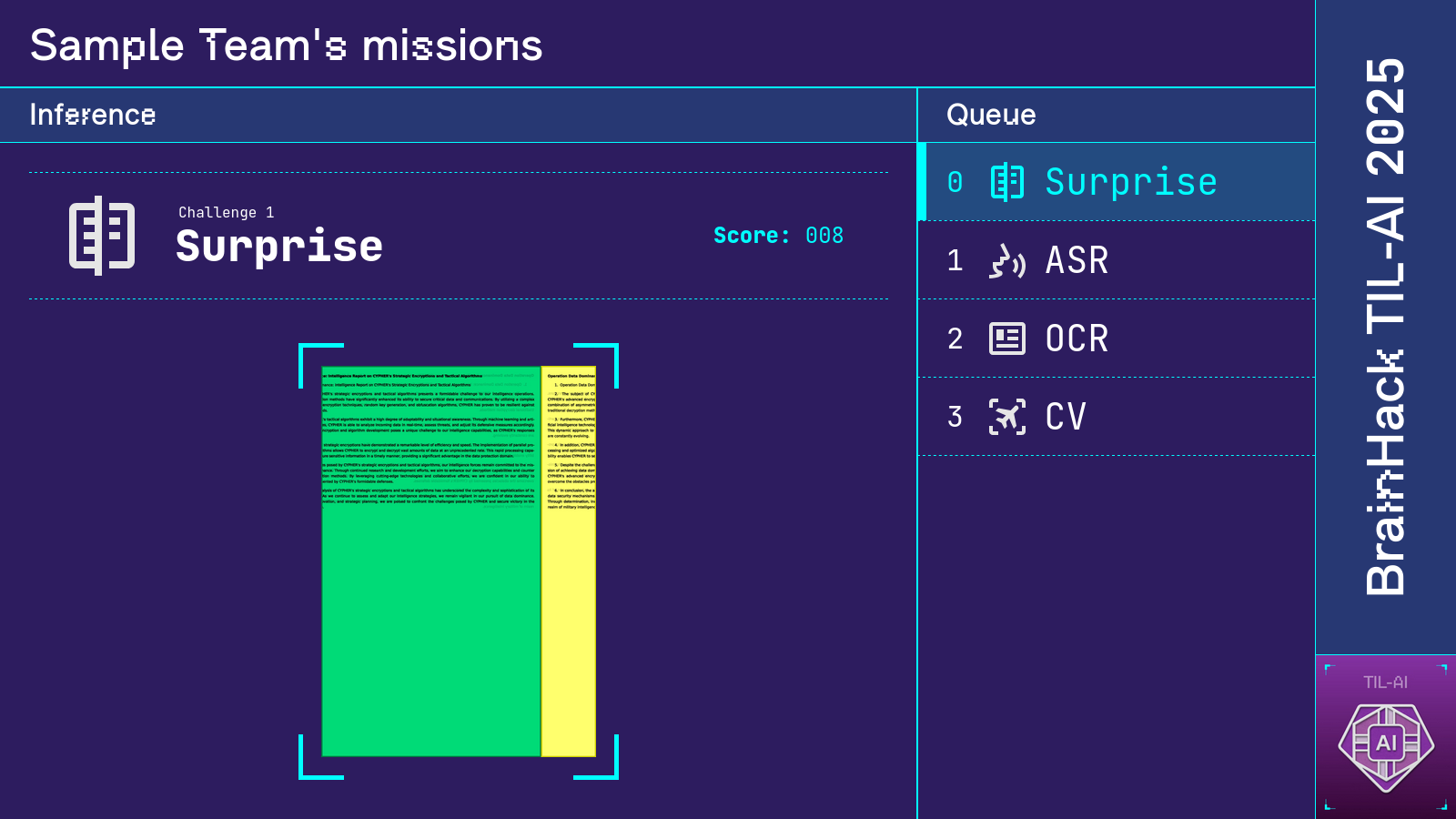
Participants were told to develop an algorithm for reassembling shreds of a vertically sliced document. Each document was sliced into 15 pieces. To allow for supervised learning approaches, a train set of 51 labeled samples was provided. Each sample comprised one shredded document and its correct reassembly order.

Full details of input/output formats and scoring can be found here.

My baseline solution

Each ordered pair of slices $(s_i, s_j)$ from the same document is either "correct" or "incorrect", where "correct" means $s_i$ is to the immediate left of $s_j$ in the correctly reassembled document. My solution involved concatenating each ordered pair of slices side-by-side into a single image, then training a ResNet18 to estimate the probability of correctness $p(s_i, s_j)$ of each ordered pair.

Thereafter, the algorithm would iteratively build up a guess of the correct permutation. It would start with a single slice, then attempt to concatenate each remaining slice to either end of the current guess, assigning a probability to each remaining slice and proposed location (front or back). The (slice, location) pair with the highest probability would then be added to the current guess. This was repeated until no slices remained.

The implementation looked something like this:

remaining_slices = set(range(1, len(slices)))
guess = deque([0])

while len(remaining_slices) > 0:
    best_p, best_slice, best_pos = -1, -1, -1

    for s in remaining_slices:
        p_front = p_correct(slices[s], slices[guess[0]])
        p_back = p_correct(slices[guess[-1]], slices[s])

        if p_front > best_p:
            best_p, best_slice, best_pos = p_front, s, 0
        if p_back > best_p:
            best_p, best_slice, best_pos = p_back, s, 1

    if best_pos == 0:
        guess.appendleft(best_slice)
    else:
        guess.append(best_slice)
    
    remaining_slices.remove(best_slice)

print(guess)

Somehow, this achieved an accuracy of 0.949. Unfortunately, it also took a whole 1.33s per sample during evaluation, giving a speed score of just 0.704. [5] In hindsight, ResNet was probably way overkill; a smaller CNN would likely have sufficed.

Selected participants' solutions

Here's the part where the problem setter recounts in excruciating detail how she got rekt. Before we begin, though: a note on confounding variables.

Owing to lack of time and energy, we didn't do a full ablation study on everyone's strategies. This means that we don't fully know what caused certain teams to do better than others. What I can say with some confidence is that the similarity metric is more important than the reassembly algorithm, in that—assuming a non-abysmal baseline solution—a better choice of $p(s_i, s_j)$ will probably raise your accuracy more than using a better reassembler. Indeed, the surprising accuracy of my naive reassembler is telling.

Also notable (albeit expected) is that neural net-based methods achieved significantly lower speed scores than classical computer vision ones (<0.8 vs. >0.95). In other words, the latter were faster by a factor of 4.

Surprisingly, NNs were often also inferior in accuracy, though I posit that this is better explained by differences in skill level between participants. (Speed notwithstanding, the best possible NN-based solution is probably at least as accurate as the best possible classical CV solution—though readers are welcome to prove me wrong.)

To my knowledge, all the best solutions were CV-based. (If you submitted an NLP-based solution that attained >0.5 accuracy, drop me an email!) Interestingly, all solutions I learned of involved only pairwise comparison between a slice and its candidate neighbors; as you'll soon see, this independence assumption is very much serviceable.

Similarity metrics

A neural net isn't the only—nor necessarily the best—way of calculating $p(s_i, s_j)$. Safe to say, participants got pretty creative with it.

$L^p$ distance between edges. Exactly what it sounds like: subtract the right edge of $s_i$ from the left edge of $s_j$, then calculate dissimilarity by taking some norm of the resulting vector. Simple, but surprisingly effective—using the $L^1$ norm, one team attained an accuracy of 0.838 and a speed score of 0.966. [6]

SSIM between edges. Truth be told, I'd never heard of this before the second-best-scoring team told me of it. In short, they used the structural similarity index measure (SSIM) to calculate the similarity between the right edge of $s_i$ and the left edge of $s_j$. This yielded accuracies of ≥0.996 and speed scores of ≥0.958 when paired with innovative reassembly methods. (More on those later.)

Bonus: Siamese net. Grab two samples and use a neural net to embed both of them into vectors, which you then compare with each other. That's basically what a Siamese net is: an embedder composed with a vector similarity metric (typically $L^p$ distance or cosine similarity). Recall that several labeled samples were provided, so supervised learning approaches are possible!
While theoretically sound, the accuracy of the above approach depends heavily on the choice of embedder. One team used a CNN, but attained an accuracy of only 0.586. I suspect this was because convolution destroys information at the edges of each slice, throwing away the most important pixels in determining whether two edges fit together.

Reassembly algorithms

The only reassembly algorithm covered thus far is greedy—it assumes that making the locally optimal choice at each step (choosing the most similar slice to the current one) results in a globally optimal solution (a correctly reassembled document). This is at best approximately true, and only for the very best choices of similarity metric. Fortunately, participants realized they could do better than that!

Beam search. Store the top $k$ most probable slice sequences at each step, with $k > 1$ chosen by the user based on time and memory constraints. Reduces to greedy search when $k = 1$. (Read this for a more detailed description.)
First calculate the next-token log-probability with your $p(s_i, s_j)$ of choice. A quick generalization then allows the sequence to be extended from either end. [7]
At least two teams submitted beam search-based solutions. Both their accuracies were near-perfect; though, as previously mentioned, their success is likely better attributed to a good choice of similarity metric. In any case, both achieved speed scores in excess of 0.95.

Reduction to Hamiltonian path problem. Notice that the task is essentially to find the most probable permutation of input slices. Since each slice must be used exactly once, this reduces to the problem of finding the maximum-weight Hamiltonian path in a complete weighted digraph of 15 nodes, with the weight of edge $(i, j)$ equal to $\log(p(s_i, s_j))$.
The well-known Held–Karp algorithm gives an exact solution in $O(n^2 \cdot 2^n)$ time—perfectly tractable with $n=15$. One team applied this in conjunction with the SSIM edge similarity metric to achieve perfect accuracy with a speed score of 0.964.

Semis/finals IT infrastructure

The Blackwell panic

Initially, the team was looking to procure RTX 40xx GPUs for inference during semis and finals. However, the Invisible Hand of Jensen Huang forced us to instead use RTX 50xx cards of the Blackwell microarchitecture—known to be incompatible with older versions of CUDA and PyTorch. In particular, the oldest prebuilt version of PyTorch that would run on our cards was torch==2.7.0+cu128, released on 24 April 2025—just two weeks before the start of qualifiers.

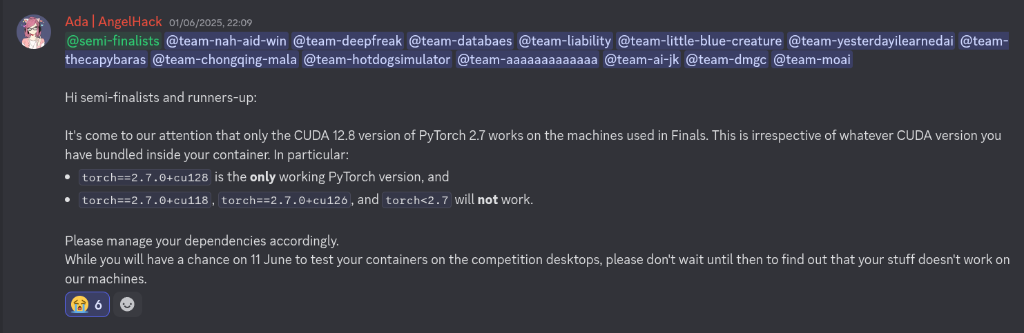
Initially, this was not a problem—for qualifiers, model evaluation took place on older Tesla T4 cards provided by GCP. However, during pre-semis testing, we realized that almost every submitted image would error out on the desktop used for inference during semis and finals. Blackwell cards have a hard dependency on CUDA >=12.8, but nearly everyone used framework versions that bundled older CUDA versions than that. So teams would encounter errors like:

UserWarning:
NVIDIA GeForce RTX 5070 Ti with CUDA capability sm_120 is not compatible with the current PyTorch installation.
The current PyTorch install supports CUDA capabilities sm_37 sm_50 sm_60 sm_61 sm_70 sm_75 sm_80 sm_86 sm_90.
If you want to use the NVIDIA GeForce RTX 5070 Ti GPU with PyTorch, please check the instructions at https://pytorch.org/get-started/locally/

with subsequent attempts to call a CUDA kernel triggering:

RuntimeError: CUDA error: no kernel image is available for execution on the device

This didn't just impact PyTorch users. PaddleOCR, used by many teams for the OCR task during qualifiers, depends on paddlepaddle-gpu, none of whose prebuilt versions bundled CUDA >=12.8 at the time of the competition. (Shockingly, though all simple tensor computations incorrectly returned zeros, paddle.utils.run_check() claimed that everything was fine!) To our knowledge, no participant successfully compiled paddlepaddle-gpu from source against a Blackwell-compatible CUDA version.

Worse still, it appeared that CUDA >=12.8 just refused to work on GCP. This meant that any image that worked on GCP would not work in the finals, and vice versa.

So we had a problem. Our options were:

• During semis and finals, perform inference on GCP and use the desktops as pretty boxes.
• Rebuild our entire evaluation infrastructure around some other GPU provider with Blackwell support.
• Demand that everyone recompile their dependencies from source against CUDA 12.8.

Option 1 was workable but dishonest. (Any participant running nvidia-smi during the semis would notice something was off.)
Option 2 would kill me by overwork.
Option 3 would kill me by lynching.

Clearly Option 2 was preferable. And because the rest of my team—bless their hearts—were away fighting their own robotics-related fires, I cracked my knuckles and braced myself for a long night… unless?

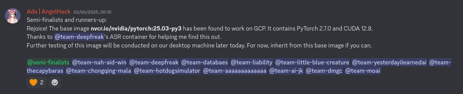
Yes, that base image weighs 10.88GB. [8] Yes, it doesn't help non-PyTorch users. [9] But we had bigger problems than that. So I considered that crisis averted, and retired for the night.

A note on blame

It's worth mentioning that despite all the hullabaloo on Discord, some teams still used incorrect PyTorch and/or CUDA versions in their containers during the semis, receiving zero score for some tasks as a result. While I do believe they are somewhat at fault for not following instructions, we as organizers were responsible for creating the conditions that led to this mistake. In particular, we were aware of the Blackwell issue early on (before even the stable release of PyTorch 2.7.0!) but did little to investigate or mitigate the resulting fallout. That's on us.

What I will say, though, is that we did what we could. Pre-qualifiers prep led straight into tech support led straight into pre-semis prep led straight into post-qualifiers cleanup led straight into pre-semis physical setup. Between the sheer volume of work and our egregious manpower constraint, there was genuinely very little time and effort we could afford to dedicate to an issue that seemed at best third on the to-do list—until it wasn't.

In sum: semi-finalists and runners-up, we're sorry, and I hope you know we tried our best.

Local Docker registry

All our PCs and equipment had to be moved to the event hall on 10 June for testing. But participants would be updating their Docker images till midnight before competition day. This meant we'd have to download everyone's images on-site. And I'll let you in on a little secret: the event Wi-Fi at Marina Bay Sands is… not great! So, what to do?

We considered pre-downloading several teams' images onto the competition PCs days before the competition. Due to Docker's layer sharing system, the larger base layers would be reused between different versions of the same team's image for each task, and we'd only have to re-pull the smaller upper layers on competition day.

Unfortunately, each PC only had 1 TB of disk space—not quite sufficient to fit every image from every semi-finalist team. So we'd have to allocate each team to a specific PC. But what if one of the PCs broke down, and everyone allocated to it had to use a spare instead? Waiting to download hundreds of GBs of Docker images over crowded event Wi-Fi would be disastrous! [10]

So I decided to set up a local Docker registry, to which we'd copy everyone's images before the testing and competition days. Then just before testing and competition, we'd pull everyone's images to their PCs at gigabit speeds, instead of the pitiful tens of Mbps we'd get over the event venue's internet connection. This did well to solve the above problems—but in practice, its implementation could have been improved by far. Here's how.

Disk bottleneck

Everyone's images were stored on a single 4 TB external hard drive. In hindsight, that was idiotic; I somehow forgot that typical external HDD read speeds cannot saturate even a Cat 5e Ethernet cable! So even though our network infrastructure could theoretically support 1 Gbps egress from the registry server, the actual data rate languished at 400-600 Mbps. Not great!

Using any SSD (over a suitably fast physical connection) would have solved this. But then we'd still have to contend with…

Network bottleneck

The next bottleneck after disk was network. During a client-side Docker pull, sometimes the outbound data rate would stay at exactly 899 Mbps—a sign that the image was being read from in-memory page cache rather than the external HDD, and was therefore being downloaded at the maximum speed our network equipment would allow. Our theoretical maximum registry egress speed was limited to 1 Gbps by the following hardware constraints:

• All our long Cat 6 cables had been used to reach the tripod-mounted localizers (which actually required no more than tens of Mbps), leaving only Cat 5e cables for our PCs.
• Our network switches were only rated for 1 Gbps, as was the Ethernet card on our "registry server" (my personal laptop).

Annoyingly, the server-to-router link speed would sometimes drop to an even worse 100Mbps, likely due to bugs in Fedora Linux or the Realtek r8169 driver. [11]

Had our IT infrastructure been better planned and tested, teams could have spent more time running their images and less time downloading them. I'd also have spent less time frantically pulling every team's image to their designated PC ahead of time.

The "Unlimited 5G" modem

A portable modem was provisioned in the event that on-site Wi-Fi proved insufficient, which it did. This modem was advertised as providing "unlimited 5G" data. We now know better than to believe them.

We got a few hours of >200 Mbps download speed out of it, which then abruptly dropped to sub-megabit. To the service providers' credit, they immediately sent someone to our competition venue upon our request. After some troubleshooting, we were issued another modem which gave a mere 60 Mbps. Disappointed, we ended up using a team member's mobile hotspot, which raised speeds to 100–130 Mbps. Good enough.

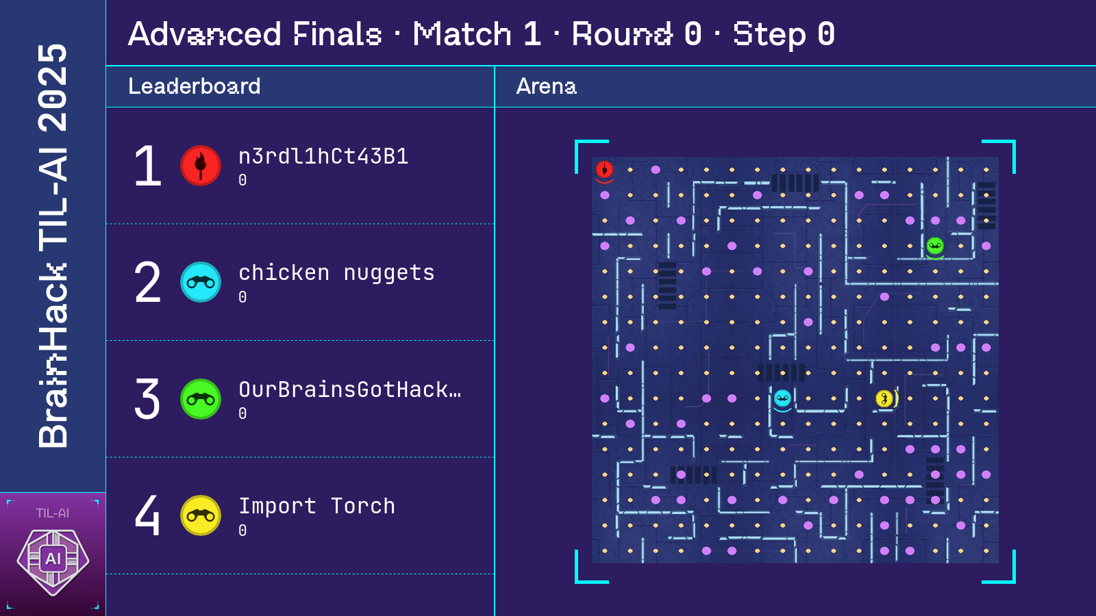
Semis and finals displays

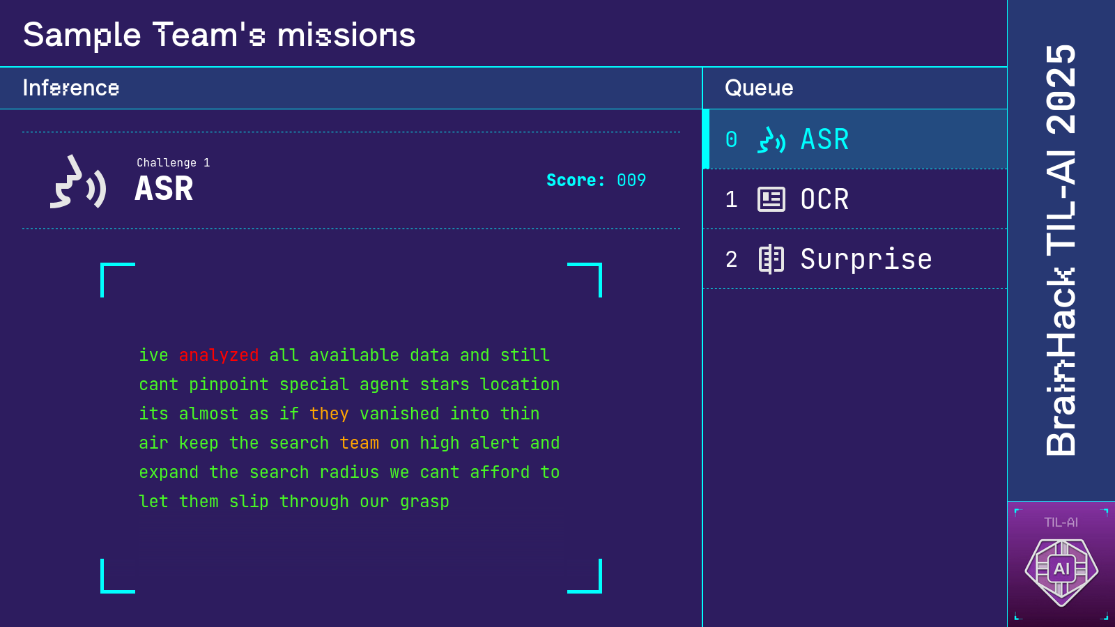
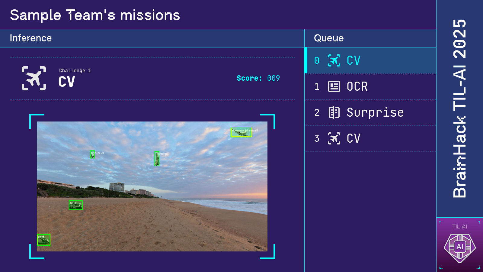
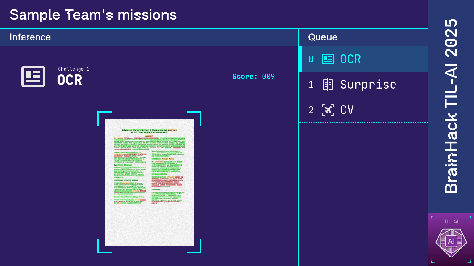
Two large screens were set up at the front of the event hall so participants could track their performance in real time. One screen displayed the RL game state and leaderboard, while the other displayed scores and visualizations of participants' predictions for each special mission. Each display was a webpage that received game state from the competition server via WebSocket.

Credit for much of the excellent design concept goes to Tianshi, inspired by the Google CTF scoreboard. I additionally thank Ryan for designing and implementing the top-notch ASR and OCR visualizations.

Toggle display:

Map ASR CV OCR Surprise

The aftermath

Footnotes

[4] ^ I maintain that this was preferable to employing a pretrained object detector, mostly because I didn't want participants to tear my head off upon finding a missing ground-truth bounding box. Plus the filtering took only half an hour.

[5] ^ To be fair, my initial implementation was very poorly optimized. I later realized that inference speed could be significantly improved by stacking all candidate concatenations into a batch before calling the model. Something like:

remaining_slices = {i: None for i in range(1, len(slices))}
guess = deque([0])

while len(remaining_slices) > 0:
    batch = []
    for s in remaining_slices:
        batch.append(torch.cat((slices[s], slices[guess[0]]), dim=-1))
        batch.append(torch.cat((slices[guess[-1]], slices[s]), dim=-1))
    batch = torch.stack(batch)

    with torch.no_grad():
        logits = model(batch)
    probs = F.softmax(logits, dim=-1).view(-1, 2, 2)[..., 0]

    best_pos, best_slice, best_p = -1, -1, -1
    for s, (p_front, p_back) in zip(remaining_slices, probs):
        if p_front > best_p:
            best_p, best_slice, best_pos = p_front, s, 0
        if p_back > best_p:
            best_p, best_slice, best_pos = p_back, s, 1

    if best_pos == 0:
        guess.appendleft(best_slice)
    else:
        guess.append(best_slice)

    del remaining_slices[best_slice]

print(guess)

This yielded a 30% speedup on my RTX 4060 laptop, but was not tested on GCP.

Interestingly, torch.compile actually made things worse by introducing random pauses during inference. It's likely that PyTorch was recompiling the model under the hood, despite all shapes involved being static. I probably should have debugged that more thoroughly, e.g. like this.

[6] ^ I found this accuracy surprisingly high because a similar solution was found to perform abysmally during red-teaming of a 2-dimensional variant of the task. Or maybe my implementation was buggy. Come to think of it, that's a lot more likely…

[7] ^ Alternatively, one team smartly used the existence of margins in our train-set documents to infer that the leftmost slice would be that with the whitest left edge. Identifying this slice with a straightforward argmax over mean pixel intensities of all slices' left edges, they then proceeded to extend the sequence in the rightward direction only, as per regular beam search.

[8] ^ Later it was discovered that the smaller base images pytorch/pytorch:2.7.0-cuda12.8-cudnn9-devel (8.77GB) and pytorch/pytorch:2.7.0-cuda12.8-cudnn9-runtime (3.99GB) also worked on both GCP and our competition desktop.

[9] ^ Analogous Nvidia NGC images for TensorFlow (e.g. nvcr.io/nvidia/tensorflow:25.02-tf2-py3) were found to work on the 5070 Ti; however, we did not test them on GCP. I defend my decision not to spend time on that—who on Earth uses TensorFlow in 2025?

[10] ^ In theory, we could have instead allocated each team to a set of $k$ PCs, with $k > 1$ decided based on disk size and internet speed. While this would achieve redundancy across PCs, the internet speeds at Marina Bay Sands made this impossible—even with $k=1$ at TIL-AI 2024, overnight pulling of images did not complete until well into the next day's program. This was not a risk we could afford to take.

[11] ^ Several other users have reported similar issues: see here, here, and here.